Price Theory for Leftists

The Canadian Centre for Policy Alternatives, a left leaning think tank based in Ottawa, published an article on February 3 titled “The numbers don’t lie: The housing crisis is not caused by a supply shortage.” The article was penned by Niko Block, a PhD student in political science at York University in Toronto. It was based on a paper that Block had written in January.

That Canada is facing a housing crisis is disputed by almost no one. That one of the chief problems is a lack of housing supply is also generally acknowledged—Block’s comments notwithstanding. Indeed, the main debate between the Liberals and Conservatives in recent years has merely been over how best to increase the supply. The Liberals see government-subsidized housing as the solution. Conservatives, on the other hand, would have governments relax zoning rules so the private sector can develop new housing. It will come as no surprise to readers of this newsletter that I strongly favor the latter approach.

But Block wants to bring the debate to a higher level. He suggests that the relative consensus on supply being the issue is misguided. Instead, he proposes that the problem is the financialization of the housing market.

Block makes a straightforward empirical argument to counter the supply-shortage position. Looking at the last fifty years, housing prices have clearly soared, and he presents data to this effect. And yet, he notes, over that same period the stock of dwellings per capita in Canada has also risen. There are more housing units per person today, when prices are high, than there were fifty years ago, when prices were lower.

Block thus writes:

The “supply-shortage argument” is encapsulated by the [Canada Mortgage and Housing Corporation’s] claim that “increasing housing supply is the key to restoring affordability.” If the argument is correct, then we should expect to see evidence that increases in dwellings per capita lower prices over time. But historical data show the opposite.

“In the face of these indicators it is not viable to argue that a supply shortage has driven housing prices up,” Block concludes. “There is no shortage of supply.”

To rebut Block’s argument, we first need to review basic price theory—what does economics teach us about how prices are formed and why they change? Of course, most people can recite the old “supply and demand” argument. And to be sure, that’s basically where we’re headed. But, to make a similar point as in my previous piece, I think most people’s understanding of supply and demand is too superficial, leaving them ill-prepared to respond confidently to arguments like the one Block is putting forward. So let’s review this theory from the ground up, getting a little more technical than usual so that we really understand it, and then I’ll show you how we can use price theory to expose the error in Block’s argument.

Price Theory 101

A price is simply an exchange ratio between two goods or services (we’ll mostly focus on physical goods for simplicity). If I give you two bananas in exchange for one apple, we can say that the price of the apple was two bananas per apple, or 2:1. When money is one of the goods being exchanged, then we are talking about money prices. If a box of cereal costs $3, then the price in terms of money is $3 per box, or 3:1.

Exchanges only take place when both parties expect to benefit, that is, when both parties value what they get more than what they have to give up to get it. The concept of value scales is thus central to the analysis of exchange. For the box of cereal, we might have the following value scales. Brackets mean the item is not currently in the person’s possession.

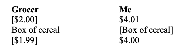
These scales indicate that I would be willing to pay up to $4 for a box of cereal, and the grocer would be willing to sell it for as little as $2. I value the box more than $4, but not more than $4.01. Likewise, the grocer values the box of cereal less than $2, but not less than $1.99.

With the scales arranged thus, there is a window between $2 and $4 where mutually beneficial exchange can take place. If we agree on, say, $3, then I am happy, because I valued the box more than the $3, and the grocer is happy, because he valued the $3 more than the box. The price we end up agreeing on is not determined except to say that it must be within this window. Where in this window it falls comes down to how well each of us bargains—our “higgling” as the Austrian economist Eugen von Böhm-Bawerk called it.

The above example is called isolated exchange, because there are only two parties. Now let’s add a number of buyers so that we have one-sided competition. Instead of writing out all the value scales, we’ll simply designate the maximum buying power of each buyer, that is, the highest price they would be willing to pay for the box. We will arrange them by their buying power for simplicity.

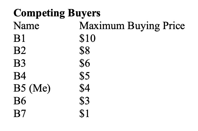
If a single grocer is faced with these buyers, what do we expect the price will be? Clearly, it cannot be more than $10, because that is the most anyone is willing to pay. But it also can’t be below $8, because if bidding started at, say, $5, B1 would bid the price up until he outbid everyone else, that is, until the price rose above the first excluded buyer, namely B2.

The only other thing we have to keep in mind is that the sole seller may have a different minimum selling price that they would accept, say, $7, or maybe $9. If their minimum selling price is $7—they would not sell it unless they could get at least that much for it—then it’s clear that the buyers will simply put the price in the $8-$10 window, all of which would be satisfactory to the seller. But if the seller’s minimum selling price was $9, then even if B1 bid $8.50, the seller would refuse. Only if the price was above $9 would the seller be willing to trade, and of course it must still be below $10 for B1 to be willing to trade.

The law for one-sided competition among buyers, then, is that the maximum price will be the highest price that anyone (in this case B1) is willing to pay, and the minimum price will be either the highest price of the first excluded buyer (B2) or the minimum selling price of the seller, whichever is higher. Within this range price is determined, as in isolated exchange, by bargaining.

Now let’s look at one-sided competition with one buyer and multiple sellers. Rather than having a maximum buying price, sellers have a minimum selling price, a price below which they would not make the trade. A group of competing sellers might have the following minimum prices. As before, we will arrange them from most powerful (i.e. most willing to trade) at the top to least powerful (least willing to trade) at the bottom.

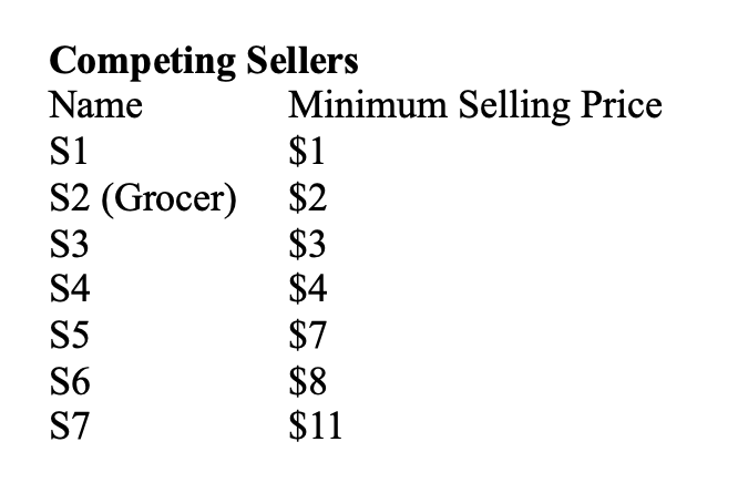
As we can see, S1 would sell the box for as low as $1, but S4 will only sell it if he can get $4 or more, S6 insists on $8 or more, and so on.

Now I come into the market as a sole buyer, willing to pay up to $4. The analysis is precisely the reverse of the previous case. At $4, S1, S2, S3, and S4 are all willing to sell, and so they start to bid the price down. Eventually, S1 says he’ll sell it for less than $2, pushing even S2 out of the market. If my maximum buying price is $4—I would pay up to $4 to get it—then it’s clear that the final price will be above $1 but below $2. If my maximum price were, say, $1.50, however, then the price range would be between $1 and $1.50. Thus, price in a market with one buyer and multiple sellers falls in a window bounded, on the low end, by the minimum price of the most capable seller (S1), and, on the upper end, by either the minimum price of the first excluded seller (S2), or the maximum price of the sole buyer (Me), whichever is lower. Within this range price is determined, again, by bargaining.

If you need to, re-read the above section so that you’re really comfortable with the logic. It’s actually simpler than it might seem at first glance, and it’s honestly kind of cool.

But the really cool part is when we have multiple sellers and multiple buyers at the same time, which is far more realistic for the vast majority of real-life markets. This is called two-sided competition.

Two-Sided Competition and the Marginal Pairs

Let’s say we have a market with seven possible sellers, each possessing one box of cereal they might be willing to sell, and seven possible buyers, each interested in one box, for the right price. Let’s further stipulate that these buyers and sellers have the maximum buying prices and minimum selling prices of our market participants in the two examples above, namely, B1-B7 and S1-S7. Since there are seven sellers each with one box, the total quantity of boxes in the market is seven, and thus that is the most that can be traded.

Here are the value scales again, for ease of reference.

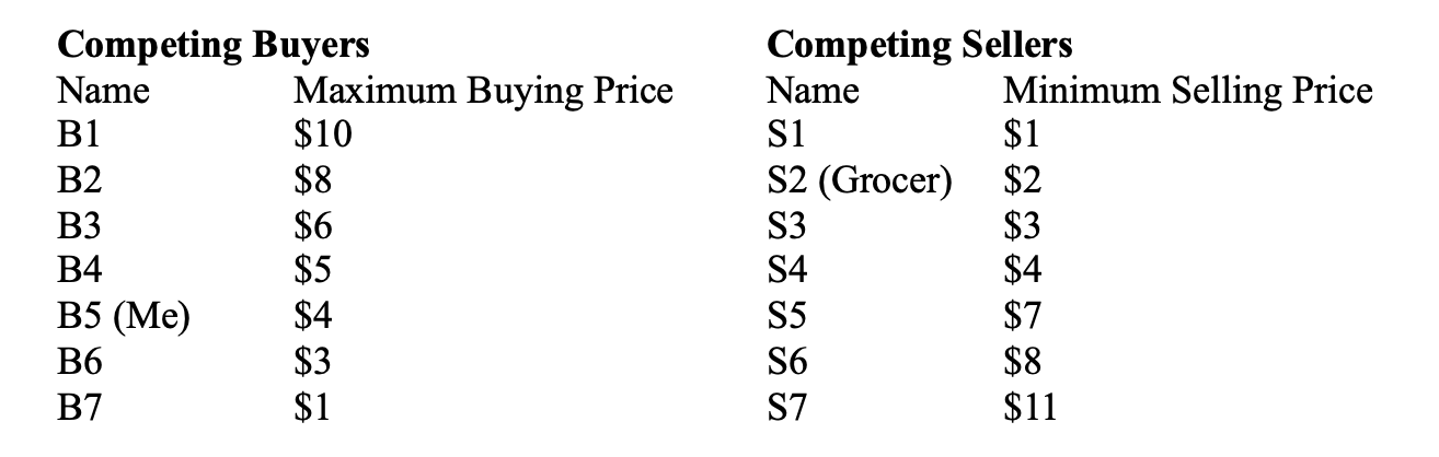
To discover the rules for price determination, let’s proceed as before, picking an arbitrary price where bidding can start and thinking through what would happen. At $2.50 per box, say, we would have two sellers interested in selling, namely S1 and S2, and six buyers willing to buy, namely B1-B6. With such an imbalance, the buyers would begin to outbid one another, pushing the price up.

At $3.50 per box, B6 has dropped out, but S3 is now ready to trade. We thus have three sellers and five buyers. Since the imbalance remains, the price continues to be bid up. If it becomes $4.50, we will have four sellers, S1-S4, and four buyers, B1-B4. Since there are four willing buyers and four willing sellers at this price, we can expect a market exchange to occur, with the four most capable sellers selling their boxes to the four most capable buyers.

The price can perhaps go a bit higher, but if it goes too high then the opposite force begins to kick in. Say we start bidding at $7.50. At this price, five sellers (S1-S5) are happy to trade, but only two buyers (B1 and B2) are interested. Noticing this competition, the sellers offer lower and lower prices, gradually knocking out sellers and bringing in buyers until a market clearing price is again reached, that is, a price where the quantity supplied equals the quantity demanded.

With this in mind, we can now ask, given the value scales of the various market participants, what is the window in which the market clearing price will fall? Perhaps a more helpful way of asking this question is: what are the upper and lower bounds of price for there to be an equal number of buyers and sellers?

Let’s start with the upper bound. There are two ways the price can get too high for the market to clear. One is if we induce another seller to come in. The other is if we knock out a buyer. We saw earlier that $4.50 is a market clearing price. Would $5.50 still clear the market? In this case, there would still be four sellers, but now there are only three buyers. B4, who was previously included, is now no longer interested. Thus, the number of buyers and sellers is not equal, and the market doesn’t clear.

Our problem could have come from the seller side, however. If the seller value scales were arranged in such a way that a new seller came in before B4 dropped out, then the new seller would cause the inequality before B4 had a chance to.

Since these individuals play a particularly important role, it helps to give them specific names, as in the previous examples. B4 in this case is the last included buyer, that is, the buyer with the lowest maximum buying price who still gets included in the market when the market clears. The other important role is the first excluded seller, which is the first seller who would jump in if the price moved above the market clearing price window. In our example, the first excluded seller is S5.

The rule for the upper bound in two-sided competition is that it is equal to either the maximum buying price of the last included buyer, or the minimum selling price of the first excluded seller, whichever is lower. In our example, B4’s maximum buying price ($5) is lower than S5’s minimum selling price ($7), and so $5 is the upper limit. The market will not clear above that price.

Now for the lower limit, which follows a beautifully parallel logic.

We begin again at $4.50, which we know clears the market. As we move down in price, we again run into one of two possible problems. Either a new buyer will be induced to come into the market, or an existing seller will be induced to leave. In either case, the quantity supplied no longer equals the quantity demanded, and the market doesn’t clear.

In our example, moving down in price yields interesting results when we get to $3.99. At this price, S4 is no longer interested, and, at the same time, B5 suddenly wants in on the action. One can imagine, of course, that if S4’s minimum selling price was slightly higher, say $4.05, then they would trigger the problem first. Likewise, if it was B5 whose maximum buying price was higher, then it would be he who determines the lower bound.

Thus, the rule for the lower bound in two-sided competition is that it is equal to either the minimum selling price of the last included seller, or the maximum buying price of the first excluded buyer, whichever is higher. In our example, these prices happen to be the same ($4), so that will be the lower bound.

Together, the two individuals who are involved with the upper bound and the two who are involved with the lower bound constitute the marginal pairs, the four people whose value scales determine the window of possible market clearing prices.

Note that, if we wanted to, we could use our above figures to create a graph showing the quantity demanded and the quantity supplied at different prices. The result would be the familiar X-shaped supply and demand curves. But I trust you’ll agree that the marginal pairs approach illustrates the concept much more vividly. Another benefit of this approach is that it highlights the centrality of the value scales of buyers and sellers in determining price.

Stock and Total Demand to Hold

“That’s all very interesting,” you might say, “but how does this help us debunk Niko Block?” Well, I’m getting there. Unfortunately, we still have a bit more theory we need to cover.

When we talk about the need to increase the “supply” of housing, we’re not typically talking about directly changing the value scales of sellers. What we really mean is increasing the physical stock, that is, the actual number of houses out there to be owned.

To support the thesis that increasing the physical stock is an important means for lowering the price, we need to have a theory that connects price with stock, and specifically one that demonstrates that more stock equals lower prices. We haven’t really done that yet, so let’s extend our analysis above to develop that theory.

Here, again, are the value scales, for ease of reference.

Looking back at our buyers and sellers, we can ask an interesting question: what is the quantity demanded at $9.50? It’s tempting to say one, namely B1, because he is the only buyer who would pay that much for a box. And there’s a sense in which that’s true. But think about S7. S7 currently possesses a box and is not willing to give it up at that price. So really, S7 has a kind of reservation demand for his box, that is, a demand to hold on to it. If we add the quantity demanded both from buyers and from the reservation demand of sellers, we get what we might call the total demand to hold, or simply total demand.

If we calculated the quantity supplied (QS), seller demand to hold (SDtH), quantity demanded (QD), and the total demand at each price, we would get the following table.

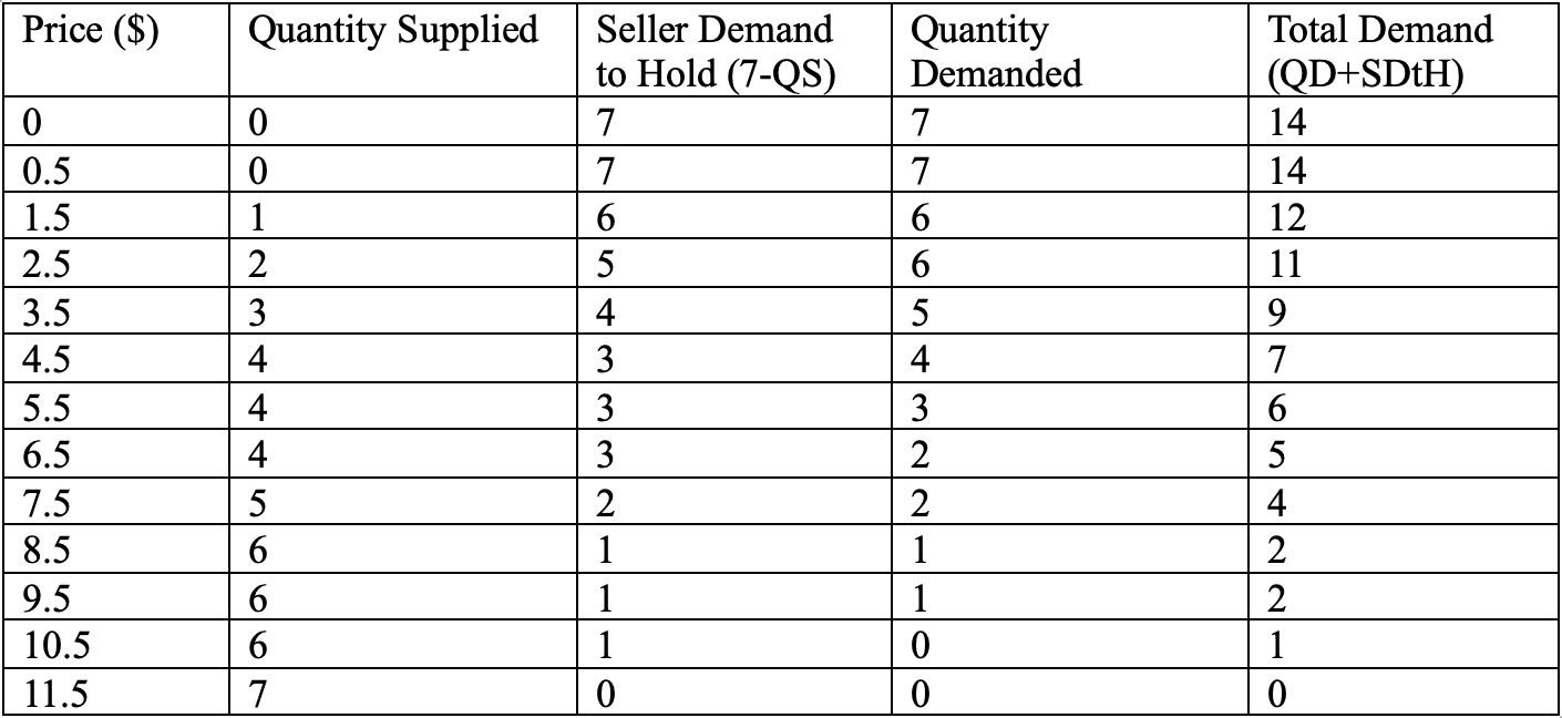
What’s interesting about this table is that in the market clearing price window, here represented by the price $4.50 (note QS=QD=4 at this price) the total demand is equal to the stock, that is, 7 units. This is not an accident. It is part of what it means for the market to clear. When the market clears the total demand for the good at the market clearing price is always equal to the amount of the good that is actually out there.

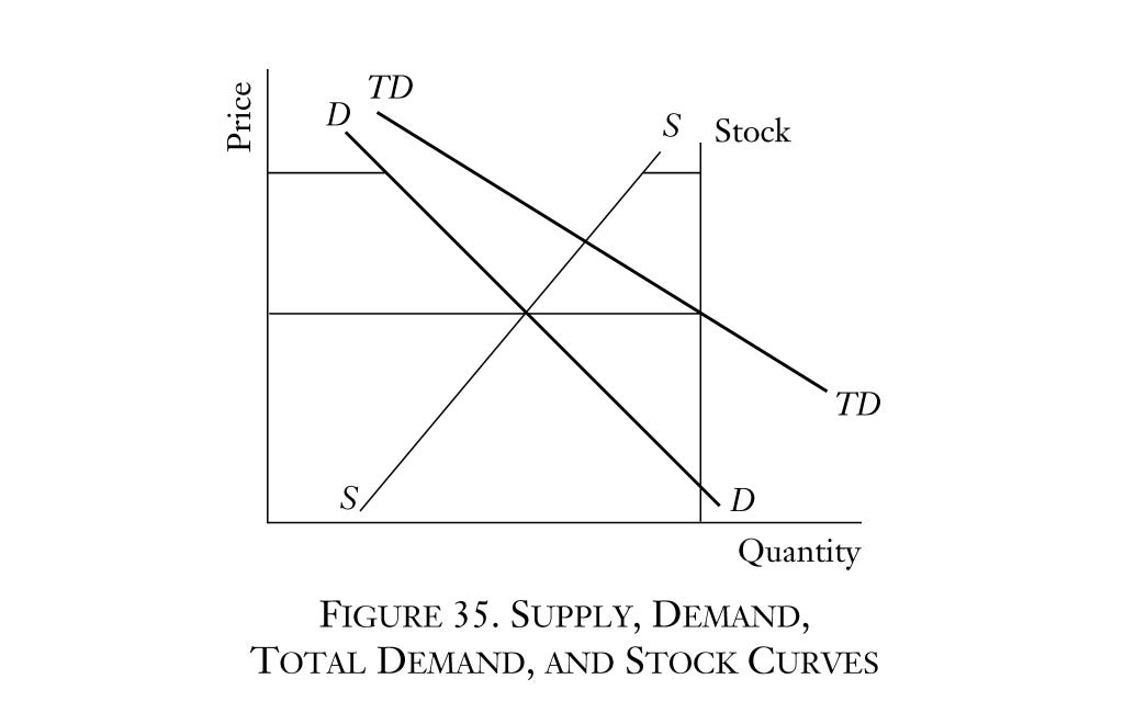
The economist Murray Rothbard illustrates this idea well in Man, Economy, and State by graphing supply, demand, total demand, and stock. Notice how supply and demand intersect at the same price as stock and total demand.

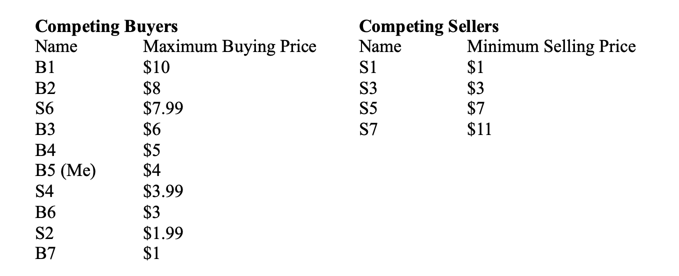
With this in mind, we can now use our theory to predict what happens when the stock changes and value scales are held constant. Say a fire destroys three of the cereal boxes, so there are only four left in the economy. Let’s say it was S2, S4, and S6 who lost their boxes. S2’s minimum selling price was $2, which means he valued the box more than $1.99 but less than $2. Now boxless, S2 becomes a buyer with a maximum buying price of $1.99. Similar changes happen for S4 and S6. Our new buyers and sellers now look like this.

Now let’s reproduce the table above for a stock of four units instead of seven.

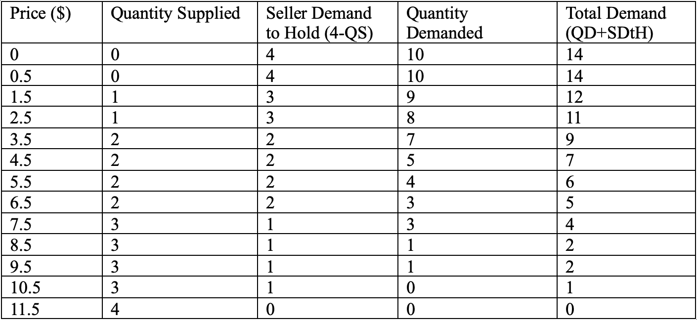
The market clearing price window is now higher, and we can see that $7.50 would be a market clearing price (QS=QD=3), and that this price corresponds with a total demand of four, which is equal to our stock. We could have determined this market clearing price simply by reading off the first table, since total demand as a function of price didn’t change, but we wouldn’t have known the market clearing quantities. Similarly, we can see that if our stock went up to, say, nine, the market would clear around $3.50, and so on.

The conclusion is inescapable. All else equal, more stock means lower prices and less stock means higher prices. This confirms our intuition, which tells us that a good which is relatively abundant will have a lower price, and a good which is relatively scarce will command a higher price.

Now we are really getting somewhere. We are starting to see why stock and price are necessarily inversely related. And, if you have a sense of where this is going, you’ll notice that we’ve already introduced the key clause that will debunk Block’s analysis. But before we can turn to that debunking, there’s one more piece of theory that the housing market in particular forces us to grapple with.

Complements and Substitutes

All of the above theory explained the market for a single good, in our case, boxes of a specific kind of cereal. If the quantity of the good is such and such, we said, and the demand for it is so and so, then here is how the price will be determined. However, the tragically misnamed “housing market” is not actually a market for the good “housing” because there is no such good. Instead, it is a series of markets for individual houses—technically plots of land—most of which people do not regard as interchangeable and thus can’t be considered to be the same good.

Is that it, then? Is the whole theory of supply and demand simply inapplicable to housing?

Not so fast.

For starters, some houses are interchangeable. Imagine a row of newly built townhomes. They are essentially in the exact same location, they are built by the same developer to the same standards in the same year. It is quite likely that market participants will regard these as completely interchangeable and develop value scales around them accordingly. Thus, it is possible to have multiple units of the same good in the realm of housing, in which case the stock and total demand analysis is completely applicable—more stock means a lower price, all else equal.

All other units of housing may not be regarded as interchangeable, but they are still economic goods with prices determined by supply and demand. The stock of these goods just happens to be one in most cases, so we are looking at one-sided competition with one seller and multiple buyers.

What’s more, while they may not be perfectly interchangeable, we can be fairly confident that individual housing units will still be regarded as substitutable. To understand the housing market, then, we need to familiarize ourselves with the economic theory of complements and substitutes.

In analyzing how prices of different goods relate to one another, economists have come up with two categories: complementary goods and substitutable goods. Complementary goods are goods that often go together, like golf clubs and golf balls. The prices of these goods tend to go in opposite directions. If golf clubs become more scarce and thus more expensive, people will golf less, causing them to demand fewer golf balls, causing the price of those balls to fall.

Substitutable goods are goods that people will substitute for one another. Different kinds of cereal would be an example. People might buy one brand of cereal instead of a different brand. In housing, people might buy one house instead of another. (Note the etymology: in-stead, which means in the place of, or “substituting for”).

The rule for substitutes is a bit more complicated (the complexity has to do with elasticity), but for many cases a reasonable simplification is that prices of substitutes rise and fall together. If Brand A of cereal becomes more scarce and thus more expensive, people will shift into Brand B, and the resulting increase in demand causes Brand B to also become more expensive. On the flip side, if Brand A becomes more abundant, resulting in a lower price, then people will demand less of Brand B, which will lower the price of Brand B.

Notably, if a completely new substitute product, say Brand C of cereal, comes on the market then the demand for Brand A will also go down as people shift to Brand C, leading to lower prices for Brand A (in this case we are no longer simplifying—this law always holds true. See p. 284 of Man, Economy, and State).

The parallels to the housing market should be clear. In most cases, each new dwelling represents a completely new product being introduced to the market. Since pretty much all dwellings in a given locale are regarded to some degree as substitutes for one another, the introduction of more individual dwellings, all else equal, reduces the demand for all other dwellings. Lower prices are the inevitable result. It is in this sense that we can say, speaking loosely, that increasing the “supply of housing” will lower the cost of housing, all else equal.

Ceteris Paribus

We are finally ready to address Block’s argument head on. Here, again, is his core claim:

The “supply-shortage argument” is encapsulated by the [Canada Mortgage and Housing Corporation’s] claim that “increasing housing supply is the key to restoring affordability.” If the argument is correct, then we should expect to see evidence that increases in dwellings per capita lower prices over time. But historical data show the opposite.

To understand what Block is doing here, let’s start with a simpler argument that’s more obviously wrong.

Say someone wanted to investigate the relationship between housing price and supply, and so they pulled data from the last fifty years on the median house price and the absolute number of dwellings in Canada. What they would find is that house prices have been steadily rising, and that the number of dwellings—the “supply of housing”—has also been steadily rising. Since the two have been increasing together, they might conclude that, whatever the relation between supply and price may be, it certainly isn’t the case that more supply leads to lower prices, as those ideological economists keep telling us.

The fallacy in this line of reasoning should be obvious. During that same time, population has drastically increased, leading to a significant influx of demand. Those pesky economists added a critical clause to their doctrine: all else equal, often expressed in Latin as ceteris paribus. The doctrine did not state that more supply would always lead to lower prices. It said more supply leads to lower prices all else equal. In other words, the impact of supply is to push price down, but if other factors, such as an increase in demand, push price up enough to more than offset this, then it is entirely possible to see more supply accompanied by higher prices. Thus, empirical data showing more supply and high prices going together do not refute the doctrine that supply exerts a downward pressure on price. They simply point to an increase in demand. If you want to isolate the impact of supply on price, you need to hold all else equal. You need to control for changes in demand.

This is what Block is trying to do by introducing his dwellings-per-capita figure. Keenly aware of the above reasoning, Block responds by saying “You’re absolutely right. Numbers that don’t control for demand tell us nothing. That is why I am looking at dwellings-per-capita.”

With a per capita figure in view, the simple objection that Block is not controlling for demand is nullified. True, population increased over the past fifty years, but if we compare, not the absolute number of houses, but the number of houses per person, then we can get a picture of how supply relative to demand has changed. If this dwellings-per-capita figure has increased at the same time as price has gone up, no one can argue that he’s not controlling for population change. He has held all else equal, he has isolated supply, and if the data show that this isolated supply has increased with price, then the economists have no answer. They must simply go back to their drawing boards and puzzle over how their theories could have been so wrong.

Such is the story that Block is trying to sell.

The critical error in this story is the assumption that population is a good proxy for demand. Block’s argument requires us to accept that controlling for population is equivalent to controlling for demand. But that is simply not the case. Demand is determined not only by the number of people in the market as buyers, but also by the intensity of their desire to own the good. Thus, demand can go up even if population stays the same. All that would be required is for people to rank housing more highly on their values scales. To be sure, demand is likely correlated to population, but it is a mistake to assume that it follows population numbers in lock step.

Since Block hasn’t controlled for demand, he isn’t really holding all else equal. True, population has grown slower than supply, but we have good reason to believe that demand has actually grown faster than supply. That reason is, of course, that prices are up! Since we know from our price theory that supply puts a downward pressure on price, we can conclude that if supply has gone up and price has gone up then demand must have gone up enough to more than offset the downward pressure of the increased supply. Indeed, the very peculiarity that Block points to in order to make his case, namely, that supply and price seem to be positively correlated even after controlling for demand, is the best evidence that his analysis didn’t properly control for demand. When you measure the sides of a right triangle and find that they don’t conform to the Pythagorean theorem, you don’t conclude that Pythagoras was wrong; you conclude that your measurement was wrong.

What is a better proxy for demand? I don’t know. Nothing will be perfect. But it also doesn’t matter, because economics is not an empirical science. We don’t need to do studies and crunch numbers to learn the laws governing prices. We can deduce them all from our armchair, as we just did above.

Why is demand up so much? I suspect it’s partly because housing is increasingly seen as a good investment, so people have become more interested in putting a lot of money in it.

Conclusion

Price theory tells us that prices are determined by supply and demand (or stock and total demand), and specifically that prices decrease as supply (or stock) increases, and that prices increase as demand (or total demand) increases, all else equal. It also stipulates that the introduction of new substitutable goods leads to lower demand and thus lower prices for their substitutes, all else equal. Applying this logic to the housing market leads to the commonsense conclusion that increasing the number of houses available is an effective means of lowering the cost of housing. This conclusion is not disproven by the data Block presents, because those data only control for population, not for demand.

There is no doubt that financialization plays an important role in the housing market. But if the left truly cares about addressing the housing crisis, they should really learn some economics and consider getting on board at least with the supply-side push, if not the YIMBY movement as a whole.

In the meantime, let it be known that elementary price theory remains undefeated.